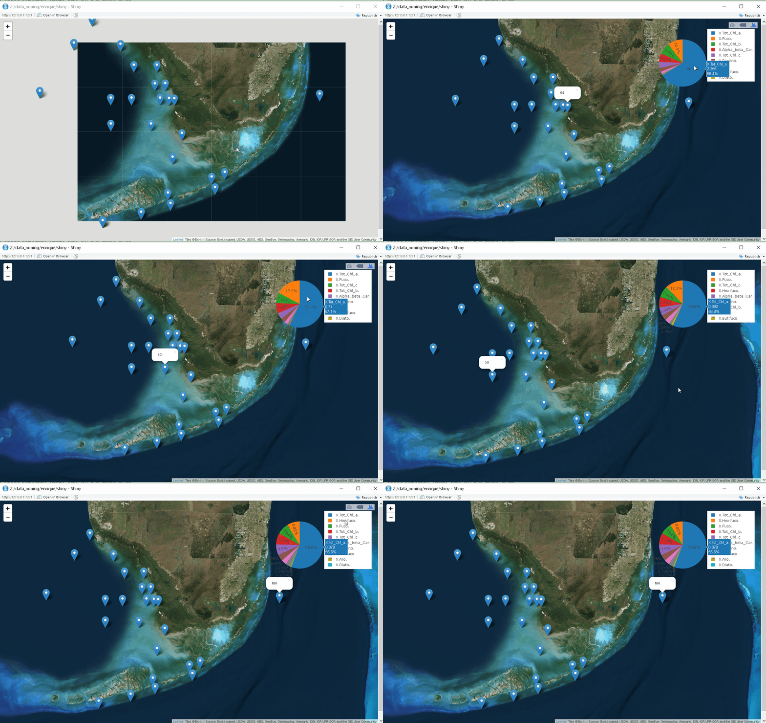
Shinyapp
09 Aug 2016One research in our lab is regarding the algae.
First they collected water samples from 58 locations around Florida Key. After collection, the samples are run through HPLC to get information about the species of chlorophylls. From those information, we would be able to know where different kind of algae lives.
To help people analysis those HPLC data. A leaflet map build with shiny server are used. The HPLC data for different stations are shown in a pie chart, which is built by plotly.

The source code are shown below and you can download them from github
ui.R
library(shiny)
library(plotly)
library(leaflet)

shinyUI( bootstrapPage(
  tags$style(type = "text/css", "html, body {width:100%;height:100%}"),
  leafletOutput("map", width = "100%", height = "100%"),
  absolutePanel(top = 10, right = 10,

                plotlyOutput("trendPlot", width = 400, height = 300)
  ),
  # this is for testing the observe
  verbatimTextOutput("Click_text")
))
server.R
library(shiny)
library(plotly)
library(leaflet)

## begin server file

# read data file
stationdata <- read.csv(file="./Muller-Karger_05-17_report.csv",head=TRUE,sep=",")
attributes(stationdata)


shinyServer( function(input, output){

  # station map
  output$map <- renderLeaflet({
    leaflet(data = stationdata) %>%
      addProviderTiles("Esri.WorldImagery") %>%
      addMarkers(lng=~Longitude, lat=~Latitude, layerId = 1:58, popup = ~Station)
  })


  observe({ # update the pie chart on map clicks
    p <- input$map_marker_click
    if(is.null(p)){
      return()
    }

    ds <- data.frame(labels = colnames(stationdata)[27:36],
                     values = as.numeric(stationdata[p$id ,27:36]))

    output$trendPlot <- renderPlotly({
      p <- plot_ly(ds, labels = labels, values = values, type = "pie") %>%
        layout(paper_bgcolor = "rgb(255,255,255,255)", plot_bgcolor="rgb(100,0,0,100)")
    })

    # this part is for testing the observe
    # text2<-paste("You've selected point ", p$id)
    # output$Click_text<-renderText({
    #   text2
    # })

  })


})
Todo List:
Add average SST(sea surface temperature) and chlor_a(chlorophyll a) data between March 13 2016 and March 20 2016 to the map.